“Flex asset value is increasingly set by tails, not averages”
Renewable capacity growth and weather-driven output swings are key drivers of flexible power asset value (e.g. BESS, LDES, interconnectors and gas plants). As RES penetration rises, the scale and frequency of output swings increasingly determine operational patterns and value capture for flexibility. At the same time, the pace and scale of RES growth drives system-wide investment requirements for flexible capacity.
Commodity prices and demand volatility also matter, underpinning price fluctuations that drive value capture for flexible assets. Stochastic modelling of RES output, commodity prices and demand provides direct insight into flexible asset value and risk – and is increasingly central to building a viable investment case.
In today’s article, we use a GB market case study to demonstrate how RES growth reshapes the distribution of power prices.
Power price distribution: GB case study
Chart 1 shows the behaviour of GB power prices in 2035, based on analysis from Timera’s stochastic power market model.
Chart 1: Distribution of Price Duration Curves in 2035
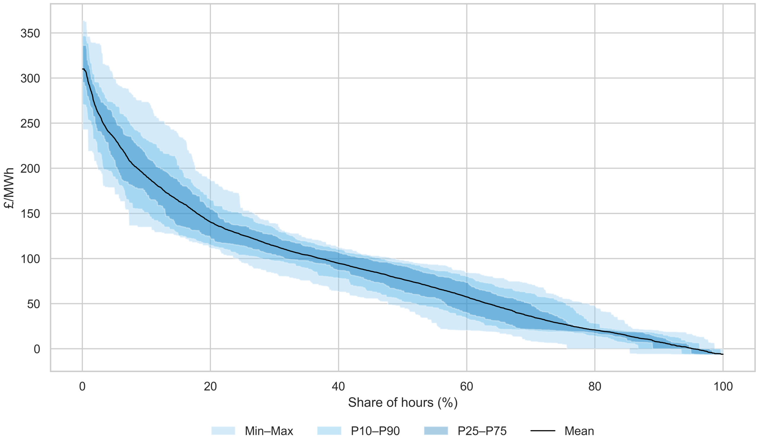
Source: Timera stochastic power market model
A Price Duration Curve (PDC) ranks all day-ahead power prices in a given year from highest to lowest, rather than in chronological order.
Chart 1 shows the distribution of PDCs from hundreds of stochastic simulations around an underlying Base case market scenario of supply, demand and commodity price assumptions. These simulations capture different correlated paths of RES output (weather uncertainty), commodity price volatility and demand fluctuations.
Key takeaways from Chart 1
- Focus on the shape, not the mean: The distribution of stochastic paths properly captures the steepness of the PDC. A steeper PDC implies wider price spreads, which translates into arbitrage and scarcity value capture (good e.g. for BESS & peakers).
- Value & risk lie in the tails: Wider percentile bands tell you price outcomes are materially uncertain even around a single path, base case scenario. Robust quantification of flex asset value and risk requires distribution-based metrics (e.g., P10, P90 revenues), not a single scenario curve.
- Correlated drivers matter: Because the distribution comes from hundreds of correlated stochastic paths (weather/RES output, commodities, demand), tail outcomes are not ‘random noise’ – they are a structural feature investors need to price.
How does RES growth impact price distributions?
In Chart 2, we model two more extreme scenarios to illustrate the impact of different RES capacity levels versus the Base case from Chart 1:
- High-RES case: additional 25 GW wind and increased CCGT retirement, with greater deployment of peakers (aligned with more bullish FES scenarios).
- Low-RES case: 25 GW less wind, reflecting stagnation in RES investment, with CCGT extensions to firm up the system.
Other generation and storage capacities are adjusted to maintain internal consistency within each scenario (e.g. lower CCGT capacity and higher engine capacity in the high-wind scenario).
Chart 2: Distribution of PDCs from High and Low RES capacity scenarios (2035)
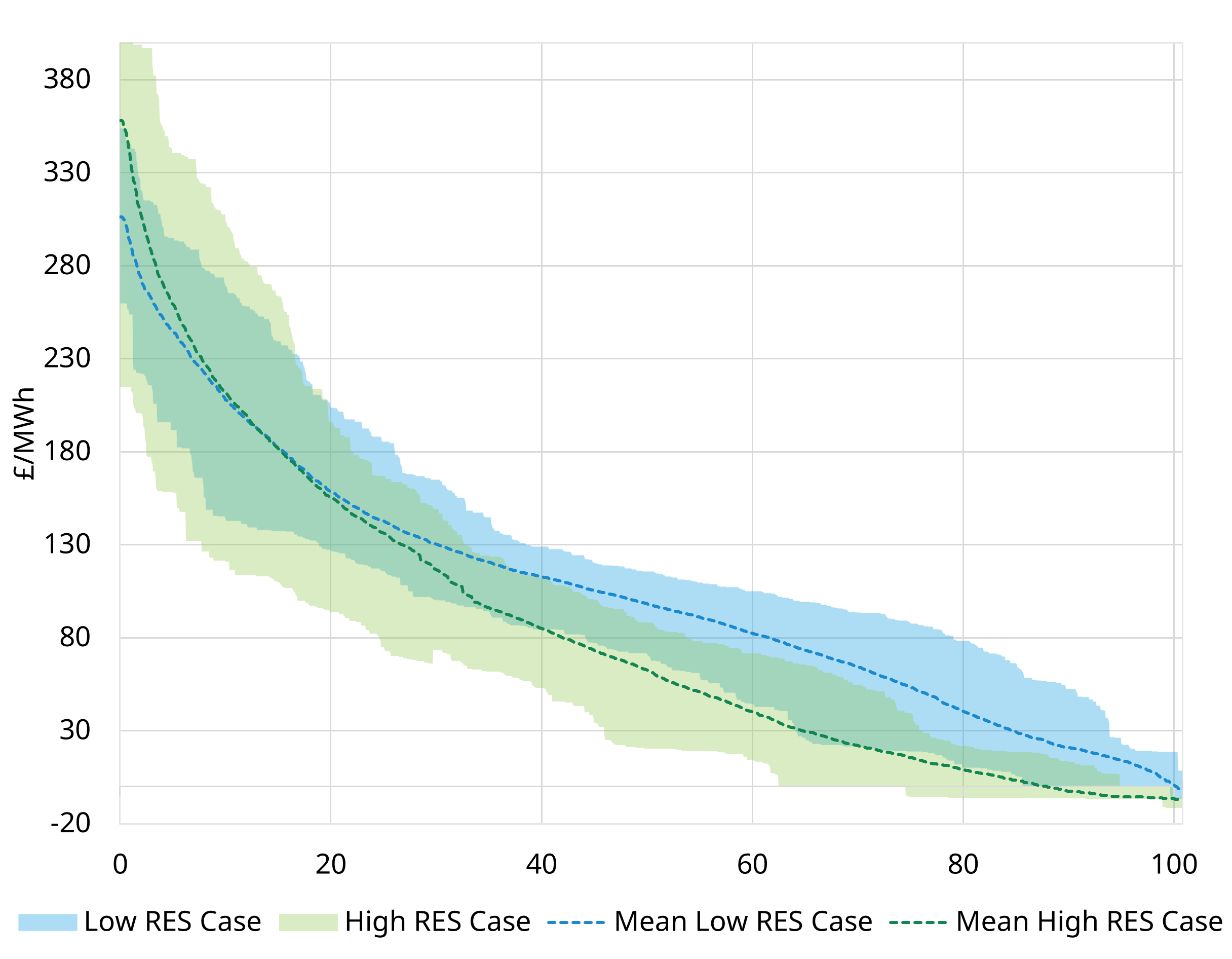
Source: Timera stochastic power market model
In Chart 2, we plot the price duration curves for all simulations in each scenario as a shaded range (min to max), alongside mean curves.
Key takeaways from Chart 2
- RES levels drive marginal pricing: average prices are lower in the High-RES scenario (greater impact of RES setting prices), relative to the Low-RES case, where the system more frequently relies on higher marginal cost plant to clear (e.g. gas peakers or storage).
- At the top end of the PDC, the picture flips: during extreme pricing periods, the High-RES scenario exhibits higher “highs” and a wider upper-tail distribution. This reflects a system with fewer alternative sources of flexibility. When RES output drops and the system tightens, high-SRMC units (typically low-efficiency peakers) are required. These assets also generally have low load factors, so scarcity pricing becomes more pronounced as they recover costs—amplifying price spikes.
- At the low-price end, the High-RES scenario is tighter: prices cluster more closely around low levels, consistent with extended periods where renewables dominate the stack and the system is persistently well supplied.
Investor takeaways across five asset classes
The stochastic price dynamics above have clear implications for flexible asset investment cases:
- BESS: High-RES systems create wider spreads and more frequent low-price periods for charging, alongside sharper high-price events during low-wind conditions, supporting arbitrage value but increasing exposure to volatility.
- Gas engines: Greater RES penetration increases exposure to low or zero prices and reduces run hours, with value increasingly concentrated in tight system events.
- Existing CCGTs: Load factors fall in high-RES systems, with value increasingly reliant on extrinsic revenues in scarcity periods.
- RES: Capture prices decline and balancing risk rises as penetration increases.
- Interconnectors: Value becomes more dependent on tail events and correlated scarcity between markets, with greater sensitivity to volatility and coincidence of tight hours.
Four ways stochastic modelling unlocks value for flex investors
Many leading investors are transitioning to stochastic analysis as RES build-out accelerates. Three reasons stand out:
1) Deterministic vs stochastic modelling
A deterministic model collapses each scenario into a single PDC, showing average shifts (e.g. High RES pushing prices down). But it provides no information on spike frequency, tail size or volatility. Stochastic modelling preserves the distribution, which increasingly drives flex value and risk.
2) Uncertainty in fundamentals drives volatility
Volatility of spot power prices is ultimately driven by short-term variability in fundamentals, such as RES intermittency, demand variability & input price volatility (e.g. gas & carbon). Modelling this directly provides a robust & superior analysis of volatility compared to traditional statistical pricing models.
3) Value is set by extremes, not averages
Asset value is often driven by tight hours and oversupply periods. By preserving real-world correlations between wind, solar and demand, stochastic modelling captures tail events that deterministic approaches smooth away.
4) Risk and optionality are explicitly quantified
Hundreds of weather-driven simulations produce a full distribution of price outcomes, translating RES uncertainty into downside risk and upside optionality for flexible assets such as BESS and engines.
If you’d like to discuss our modelling approach in more depth or our views of GB and European power markets, feel free to reach out to Arshpreet Dhatt (Senior Analyst) arshpreet.dhatt@timera-energy.com.