Everyone is familiar with the Base, High & Low scenario approach to power market analysis. This is rooted in common sense. What is our best guess of what could happen (Base)? How could we be wrong (High & Low)?
However, the large scale roll out of intermittent renewable capacity in power markets has undermined this traditional scenario approach. The inherent uncertainty of wind & solar output patterns and the substantial range of volume swings requires something new.
Probabilistic (e.g. simulation) based analysis of power markets is needed to properly understand:
- The distributions of potential market outcomes (both prices and volumes)
- The risk/return distributions of individual assets operating in those markets.
In today’s article we use a UK power market case study to illustrate how power market uncertainty can be deconstructed and analysed. We look at some of the key market impacts of higher renewable penetration on market prices and asset values.
Why the traditional approach is broken
Traditional power market modelling involves creating detailed deterministic scenarios (e.g. Base, High, Low), that model a power system under a fixed set of conditions.
These deterministic scenarios are based on ‘average’ or ‘historical’ conditions for key sources of uncertainty in the market, for example:
- Intermittent solar and wind output
- Demand (e.g. short-term deviations due to weather).
This deterministic approach may have been adequate when these sources of market uncertainty were in aggregate not large enough to have a significant impact on price & volume outcomes. But the large scale roll-out of renewables is changing that.
As a result, it is important to specifically capture uncertainty within the market modelling process, to understand market and value dynamics. Important examples of issues that cannot be properly dealt with via the traditional scenario approach are summarised in Table 1.
Table 1: examples of where traditional modelling breaks down
It is in the interests of asset owners and investors to properly account for uncertainty. Applying traditional scenario analysis to flexible assets such as gas peakers or batteries, typically undervalues optionality. It can also significantly misrepresent the risks around price cannibalisation for renewable assets.
Deconstructing the impact of uncertainty
Commodity prices have historically been the largest source of power market uncertainty. They remain a key driver, but for the purposes of today’s article we focus on the impact of uncertainty from wind output, solar output and demand.
Each of these three factors (wind, solar & demand) has its own unique behavioural characteristics. But these can be aggregated to generate a combined distribution of net system demand (= demand – wind output – solar output).
Net system demand is effectively what the dispatchable portion of the power market supply stack must cover in order to clear the market. Chart 1 illustrates a distribution of UK net system demand overlaid on the dispatchable (or controllable) portion of the supply stack.
The chart shows the portion of time that different sections of the supply stack are required to clear net demand. For example:
- High load & low wind/solar periods in the right tail of the distribution result in peaking units setting prices
- Low load & high wind/solar periods in the left tail result in renewable or must run capacity setting zero or even negative prices.
The chart illustrates the foundation of a probabilistic approach to supply stack modelling. Multiple simulations of net system demand can be run through the stack model to generate distributions of market price & volume outcomes. These then allow analysis of the impact of net demand uncertainty on asset value (e.g. some of the drivers outlined in Table 1).
Analysing market evolution: UK case study
In Chart 1 we show the relationship between net demand and the supply stack at a given point in time. But from an asset investment perspective it is important to understand how a power market will evolve over at least 15-20 years (i.e. a capital payback horizon).
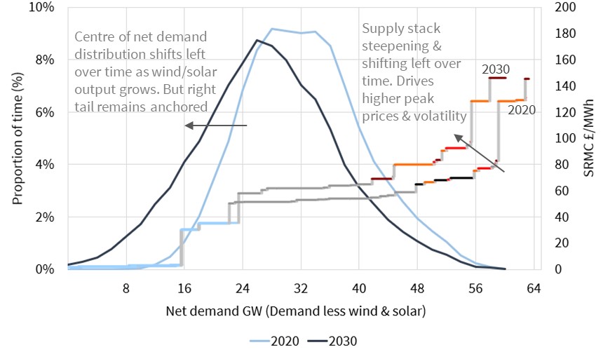
Chart 2 shows the evolution of both the dispatchable supply stack and net system demand distributions for the UK power market in 2020 versus 2030.
Chart 2 illustrates two key themes summarised below.
- Increase in wind & solar output
- Growth in wind & solar output shifts the center of the net demand distribution left over time
- But the right tail remains anchored around the level of peak demand (i.e. there are still periods of very low wind & solar output that need to be covered by peaking flex)
- The net demand distribution widens over time reflecting the increasing range of wind & solar fluctuations e.g. ~17GW wind & ~14GW solar intraday swing ranges by 2030.
- Stack steepens
- The supply stack steepens over time as (1) coal & older CCGT plants retire from the middle of the stack and (2) they are replaced by higher variable cost peaking flex to the right of the stack (e.g. batteries, engines, GTs, DSR).
- The steepening of the stack, increases the price impact of wind & solar fluctuations, i.e. output swings can tip the market from negative prices to 100+ £/MWh across several hours
- The impacts of rising battery and demand side flexibility are substantially outweighed by swings in wind & solar output
- In summary, ‘wind trumps batteries’ i.e. battery capacity (e.g. 4-6 GW by 2030) is much smaller than wind/solar swing volumes (30+ GW by 2030).
It is analysis of the interaction between changing supply and demand distributions that shines the light on how power markets will evolve. Uncertainty may be an inconvenience for asset owners & investors, but capturing it underpins the meaningful analysis of asset value dynamics. Applying the traditional Base, High and Low scenario view is a bit like trying to find a black cat in a dark room.