The LNG market has swung from covid bust to crisis explosion across the last 3 years. This period represents one of the most savage bouts of price volatility in commodity market history.
“Ultimately we care about price dynamics because they drive asset value & risk”
To put it bluntly – traditional Base / High / Low price forecasting analysis was of limited use!
It was next to impossible to forecast market swings of the scale of 2020-23. But insightful market analysis is not about precise predictions… it is about applying an analytical framework that confronts market uncertainty and provides quantitative conclusions on what could happen.
Take a simple example. At the start of 2022 it was very difficult to forecast the scale & timing of Russian supply cuts. But it was quite possible to undertake structured analysis of the impact on price levels & volatility for a given volume of supply cuts and therefore the impact on asset values.
In today’s article we set out a framework for quantifying LNG market price dynamics across the next 10 years, and use charts to summarise the evolution of pricing dynamics.
Supply flexibility: lumpy but large
In last week’s articles we set out a summary of the supply & demand volume balance across the next 10 years. Today we analyse the ‘stack’ of market flexibility that drives pricing dynamics. By this we mean the price responsiveness of different sources of supply & demand flexibility that act to clear the LNG market.
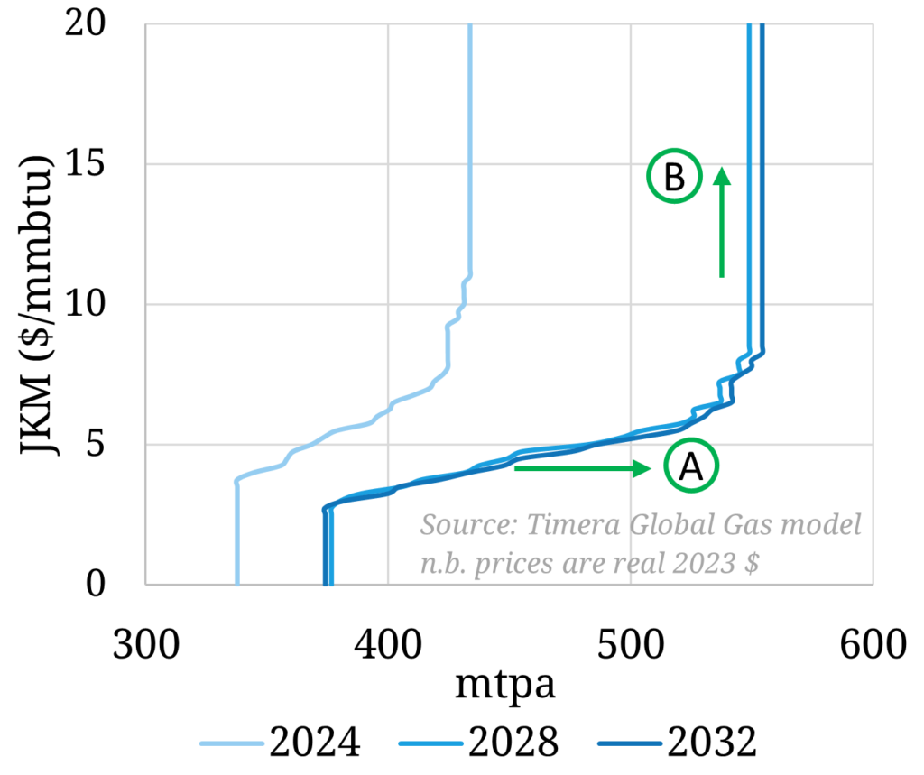
Let’s start with supply because it is a bit simpler than demand. Chart 1 shows a view of LNG market supply curve evolution in 4 year steps from 2024 to 2028 to 2032.
Chart 1: LNG market supply curve evolution
Source: Timera global gas model
These supply curves are outputs of Timera’s global gas market model. There is a lot of detail in the model behind individual liquefaction site flexibility, but there are two key high level takeways:
A. US exports are a key source of flex (see upward sloping section of curve marked A on chart)
- They represent high volumes of US hub indexed cargoes that can be cancelled if netback prices fall below variable cost (note this sloped section of the supply curve is broadening as more US capacity comes online).
- There is a ‘merit order’ of US cancellations reflecting different cost structures across US offtakers (e.g. sunk shipping costs, related portfolio sales, variable cost of feed gas).
B. Supply is otherwise very inelastic (see vertical sloping section of curve marked B on chart)
- Very limited short term ability for supply to respond to price signals given liquefaction trains operating at full capacity.
- There is however some limited supply side optimisation potential e.g. variation on timing of maintenance.
To summarise supply side response: within a 5 year lead time horizon there is very limited supply response beyond US export cancellations at lower price levels. That is why demand flex is so important in driving pricing dynamics.
Demand flexibility: less responsive & shifting to Asia
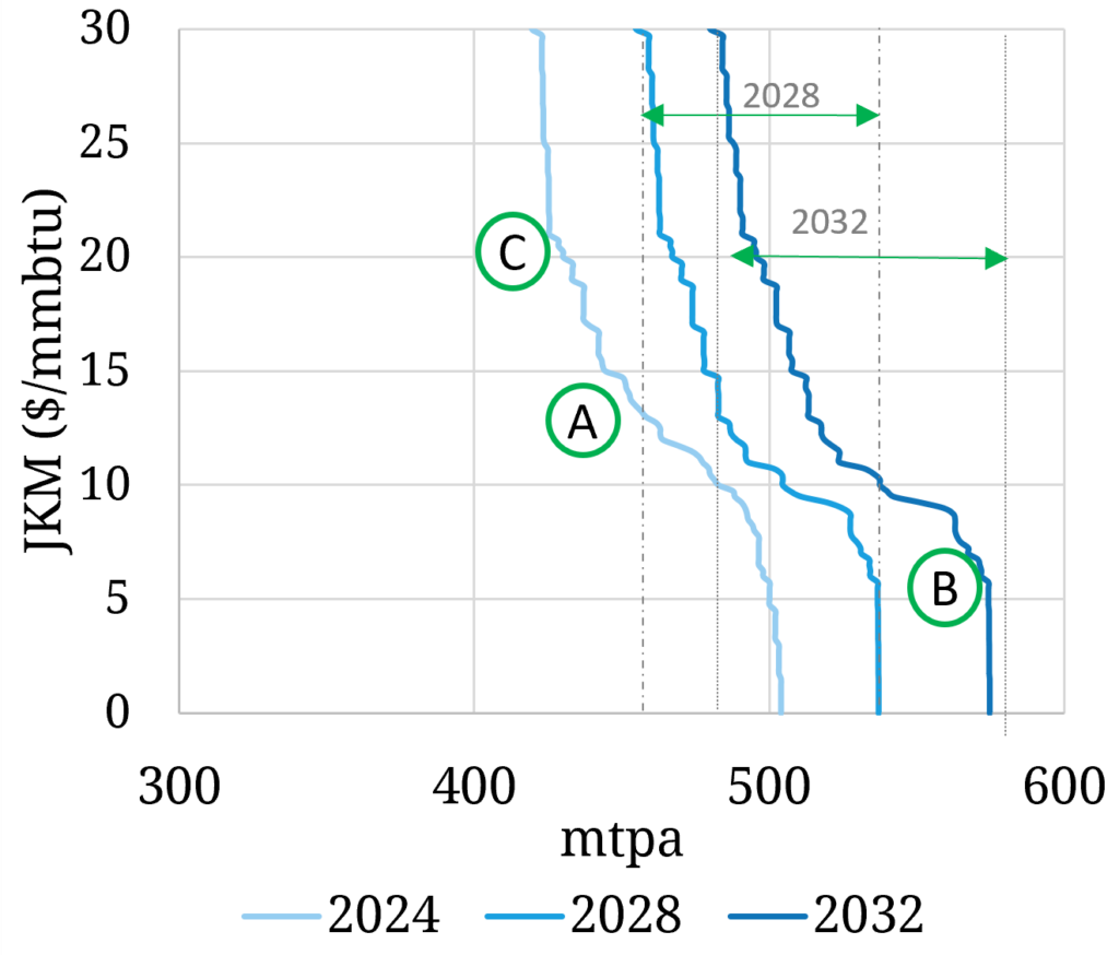
Chart 2 shows a view of LNG market demand curve evolution in the same 4 year steps as Chart 1.
Chart 2: LNG market demand curve evolution
Source: Timera global gas model
Again these supply curves are an aggregate view of a lot of complex & granular sources of demand response. But there are 3 sources of flex that play a key role in driving market pricing:
A. European coal to gas switching – liquid power markets provide real time gas demand response driven by coal & carbon price levels, playing an important role in anchoring European gas & global LNG market pricing (albeit declining significantly this decade as coal plants close).
B. Asian switching – in the form of (i) gas to oil switching (ii) pipeline vs LNG switching and (iii) power sector switching (all of which are less dynamic than European power switching).
C. Outright demand induction (at low prices) & demand destruction at high prices (at high prices) e.g. from industrial demand.
To summarise demand side response: dynamic European power sector switching has historically anchored the LNG market and dampened price volatility (with the notable exception of 2022). Going forward the LNG market is going to depend much more on less responsive Asian switching response. That means higher price volatility.
Putting the pieces together to map the way forward
In chart 3 we show the overlay of supply and demand curves for each of the focus years (2024, 2028, 2032).
Chart 3: Evolution of supply & demand curve intersection across next 10 years
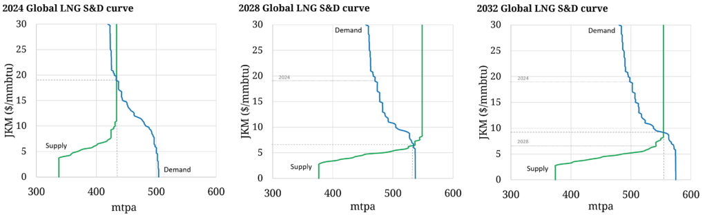
Source: Timera global gas model
Again lots going on but even at this aggregate level there are some powerful conclusions on market pricing dynamics. We summarise these in the table below bucketed by the 3 phases of LNG market evolution we set out last week.
How does this inform decisions?
Ultimately we care about price dynamics because they drive asset value & risk.
The framework we summarise above helps to understand how price levels may evolve across the next 10 years. But more importantly it helps define the prevailing price dynamics across different market regimes. For example price volatility behaviour, correlation of LNG prices vs gas hubs / Brent / coal and the impact of market shocks to the downside & upside.
We use our global gas model to drive:
- Scenario analysis – impact of different S&D outcomes e.g. stronger Asian demand
- Sensitivity analysis – market shocks e.g. Russian regime change & return of supply
- Simulation analysis – simulating distributions of hundreds of price outcomes to capture uncertainty of market evolution.
The common goal across all of this market analysis is to feed it through our LNG asset & portfolio models to quantify the impact of market evolution on value & risk and support clients with portfolio origination, investment & strategy decisions.
If you would like to find out more on our conclusions on LNG market evolution and its impact on asset value, feel free to join our ‘What’s next?’ webinar on LNG market evolution (see details below).
Join our upcoming webinar
Title: “What next?” – a framework for analysing LNG market evolution & portfolio value drivers in a post-crisis world
Date: Wed 14th Jun 09:00 BST (10:00 CET, 16:00 SGT)
Registration link here, free to attend
Focus:
- Market regime framework for price evolution to 2035
- Downside risks e.g. 2023 and 2026-28 vs potential re-tightening e.g. 2024-25
- How marginal pricing dynamics are shifting post-crisis (e.g. JKM vs TTF vs DES NWE)
- Why price volatility is structurally increasing
- Implications of new market dynamics for LNG portfolio value (e.g. US tolls, regas, shipping)